author:	ywen666
score:	10 / 10

Motivation

When optimizing a neural network whose inputs are high-dimensional, most features are zero while the infrequently occurring non-zero features are highly informative and discriminative.

To emphasize infrequently occurring features, previous algorithms follow a predetermined scheme which is oblivious to the characteristics of the training data.

This paper proposed to incorporate the geometry of training data, giving frequently occurring features low learning rates and infrequent features high learning rates. This allows the model to take more notice on predictive but rare features.

Method

This paper considers a projected gradient descent training scenario. Assuming the gradient is \(g_t\), and we want to update \(x_t\) in the opposite direction of \(g_t\) while maintaining \(x_{t+1}\in \mathcal{X}\). Generally, \(\mathcal{X}\) is the convex set over which \(x_t\) is to be minimized. And the learning rate is \(\eta\). The update at timestep \(t\) is (finding the closest point in \(\mathcal{X}\) to the ordinary gradient descent update), \(x_{t+1} = \arg\min_{x\in \mathcal{X}} || x - (x_t - \eta g_t) ||_2^2\)

I summarize this algorithm (Adagrad) in the simple case. Assuming we want to update the weights of a neural network \(\theta\), which is high-dimensional. Let \(g_{t,i}\) denote the \(i^{th}\) dimension of the gradient vector \(g_t\). The SGD update for every parameter \(\theta_i\) at timestep \(t\) is

\[\theta_{t+1, i} = \theta_{t,i} - \eta \cdot g_{t,i}\]

We want to make \(\eta\) adaptive – changing \(\eta\) at each time step t for each parameter \(\theta_i\) based on the history. We can define an outer product matrix \(G_t = \sum_{j=1}^t g_jg_j^T\).

For example, if \(i^{th}\) feature has zero gradient most of the time, then the value of it in the diagonal matrix \(diag(G_t)_i\) is small. With this diagonal matrix, we can make \(\eta\) adaptive,

\[\theta_{t+1, i} = \theta_{t,i} - \frac{\eta}{\sqrt{diag(G_t)_i + \epsilon}} \cdot g_{t,i}\]

\(\epsilon\) is the smoothing term that avoids division by zero. The inverse square root is coming from the natural gradient descent algorithm in the convex optimization.

In the vectorized form, \(\theta_{t+1} = \theta_{t} - \frac{\eta}{\sqrt{diag(G_t)+\epsilon}} \cdot g_{t}\)

With Adagrad, we don’t need to tune the learning rate (there is still a base learning rate \(\eta\), generally set to 0.01). One potential problem is that the accumulation of \(diag(G)\) with time is always positive, it might cause the effective learning rate to shrink to 0, leading to no update at all.

Notice that this summary only reflects the simpliest application of the proposed algorithm. This paper considers settings in online learning and projected gradient descent, along with very solid theoretical analysis.

Experiments

• Dataset
  • Reuters RCV1 text classification
  • MNIST multiclass digit recognition
  • Census income dataset from UCI
• Text Classification
  • RCV1 data has 4 categories Economics, Commerce, Medical, and Government (ECAT, CCAT, MCAT, GCAT)
  • Input features are 0/1 bigram features, leading to sparse feature vectors.
  • RDA and FB are two common online learning algorithms. Adding Adagrad to them improve test set error as illustrated in the table.

	RDA	FB	ADA-RDA	ADA-FB
ECAT	.051	.058	.044	.044
CCAT	.064	.111	.053	.053
GCAT	.046	.056	.040	.040
MCAT	.037	.056	.035	.034

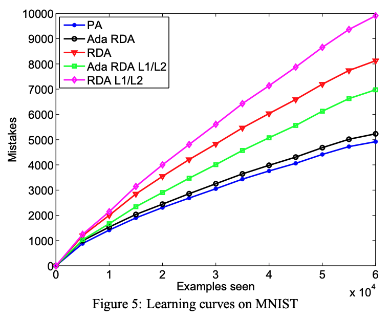
• Multiclass MNIST
  • On this dataset, his paper compared the adaptive RDA with and without mixed-norm l1/l2, RDA, and multiclass Passive
  • Aggressive to one another using the multiclass hinge loss. For each algorithm, we used the first 5000 of 60,000 training examples to choose the base step size.

RDA has significantly higher sparsity levels (PA do not have any sparsity). Naturally PA has a better accuracy than RDA.

• Income Prediction
  • The data consists of 40 demographic and employment related variables which are used to predict whether a person has income above or below $50,000.
  • They preprocessed the data into 0/1 features.
  • The table demonstrated that the test error v.s. the proportional traininig data in the online learning setup.

Prop. Train	0.05	0.1	0.25	1
PA	.049	.052	.050	.048
RDA	.055	.054	.052	.050
Ada-RDA	.053	.051	.049	.047
l1 RDA	.056	.054	.053	.051
l1 Ada-RDA	.052	.051	.050	.049

TL;DR

This paper proposed adaptive gradient descent algorithm – AdaGrad. The learning rate is adjusted based on the history of the gradient. Its most effective application is sparse feature learning.